Repeat customers can be considered as the key players of a settled and profitable business. Repeat customers help us to get more purchases without needing to acquire new ones. Repeat customers are easier to gain a trust from. Repeat customers even help us to acquire more first time buyers.
Acquiring new customers might cost higher than making the existing ones to purchase more. Even so, the latter seems to be more difficult. Business actors need to formulate when is the right time to appeal an existing customer to make his/her next purchase.
Given a customer has made a purchase once, for example, how long one should wait for him/her to make the second one. By estimating when the second purchase will be made, it might be easier to measure how challenging it is to expect more purchase from someone.

Source: starecat.com
Let’s simulate this question with a Survival Analysis.
Survival analysis was usually done to estimate lifespans of individuals (e.g. in medical prognosis). We define an event as “death”, which we want to anticipate the time of its happening at someone’s life. We’d like to measure how long someone will “survive” since “birth” until meeting his/her “death”.
The measurement comes in the form of probabilities, so one of the questions we can ask is, “What is the probability of surviving until the time \(t\)?” (e.g. until the \(t^{th}\) day after “birth”).
One example: if we define “death” as “death by heart attack at any time \(t\)” and “birth” as “observation by the doctor is started”, we can try to answer such questions like
- “What is the probability of not having a heart attack until the \(t^{th}\) day after the first observation day?”, or
- “What is the probability of having a heart attack at \(t^{th}\) day after the first observation day?”.
We actually can do survival analysis in many problems in general, as long as we adjust first how we define the “death”, “birth”, and “survive” event. We can also define how we will measure this “lifespan” by our own.
For our current context, we define
- “birth” as the event that a customer made his/her first purchase
- “death” as the event that a customer made his/her second purchase
- “lifespan” as the time difference between “birth” and “death” (or how long should we wait for a customer to make his/her second purchase).
We are using this online retail dataset that contains real transactions of gift products business in 2010 and 2011.
Lifetime Plot
Let’s observe the lifetimes of some customers.
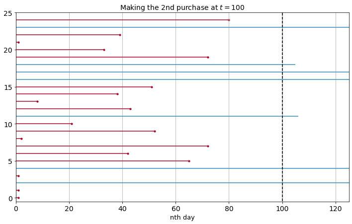
The plot above simply shows the time difference between someone’s first and second purchase. The dotted line at \(t = 100\) means we’re observing their “lifespan” until the 100th day after the first purchase. Like, how often we see a customer who made his/her second purchase in 100 days after his/her first one.
Red line means their second purchases are observed at the 100th day after the first purchase or earlier. Blue line means their second purchases haven’t observed yet in 100 days after the first purchase, implying their second purchase could be happening at the 101st day or 105th day after the first purchase, or not happening at all.
Note that some blue lines can be not too long, but some can be very long beyond the right border of the plot (the upper limit of the x-axis is adjusted on purpose to simplify the plot). We’re calling these blue lifetimes as right-censored.
Why are the right-censored data matter to notice? If we’d like to take the average “lifespan” of our customers when we’re observing them at time \(t\), the average can be underestimated by the lifespan of customers whose second purchase aren’t observed yet. We don’t know yet whether they will make second purchase beyond at time \(t\). In other words, having observed their actual lifetimes beyond time \(t\) can’t be useful in this case.
In survival analysis, we want to get a better estimation of waiting time between a customer’s first and second purchase.
Survival Function
First, let’s define a curve called survival function \(S(t)\) written down as
\[S(t) = Pr(T > t)\]
If you’re already familiar with probability density function, notation above is similar with “the probability that an event is happened after time \(t\)”. We can alter the phrase to “the probability to survive from an event until time \(t\)”. The interval between the beginning of time (“birth”) until a particular time the event is happening is our “lifespan” here, while the event can be the “death” we have defined before. So, we’d like to find what is the chance that our lifespan is beyond time \(t\).
The survival function above is also a complement of “the probability that an event is happened before or at time \(t\)”, written as \(1 - Pr(T \leq t)\).
Regarding the right-censored data issue mentioned above, we will rather estimate the survival function with something called Kaplan-Meier estimator.
\[S(t) = \prod_{i=0}^{t}1-Pr(T=i|T \geq i)\]
With notation above, we’d like to multiply the complement probabilities of death occuring at \(i\) given surviving up to time \(i\), for every \(i\) from 0 to \(t\). In our context, it’s the same as multiplying the probabilities of not making the second purchase at time \(i\) given the customer hasn’t made the second purchase up to time \(i\).
\[1-Pr(T=i|T \geq i) = 1-\frac{d_i}{n_i}\]
\(d_i\) is the number of customers who made their second purchase at \(i^{th}\) day after their first purchase, and \(n_i\) is the number of customers who haven’t made their second purchase up to \(i^{th}\) day after their first purchase.
Thus, what we need to calculate is
\[S(t)= \prod_{i=0}^{t}1-\frac{d_i}{n_i}\]
Now, it’s just a matter of multiplying a bunch of fractions.
We will use Kaplan-Meier estimator to see how many percent of customers who still haven’t made their second purchase until time \(t\). With the help of lifelines, we just need the observed “lifespan” of each customers and whether second purchase was occured at the end of their “lifespan” to get our survival function.
| |
Lifespan |
Death |
| 0 |
326 |
0 |
| 1 |
9 |
1 |
| 2 |
2 |
1 |
| 3 |
84 |
1 |
| 4 |
253 |
1 |
| 5 |
215 |
0 |
Note that since the time when a customer made their first purchase is varied, the “lifespan” of customers who haven’t made their second purchase until the end of observation can also be varied, although here we assume the end of our observation is fixed, which the last purchase date.
Here’s the plot based on our estimated survival function.
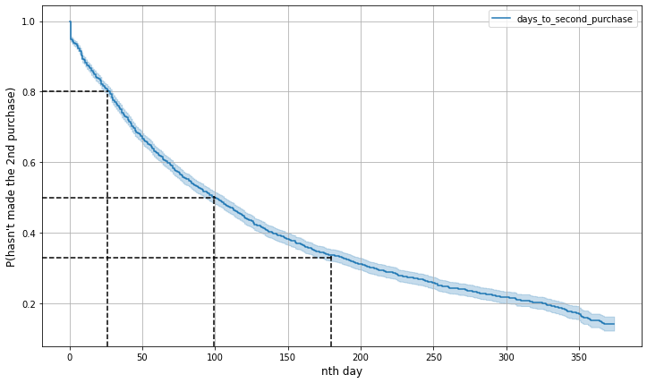
The percentage on y-axis can be seen as the probability of someone not making his/her second purchase yet until time \(t\).
What do we get here?
- Around 80% of customers haven’t made their second purchase until the 26th day after their first purchase.
- Around half of customers haven’t made their second purchase until the 99th day after their first purchase, which is around three months.
- Around 67% of customers have made their seceond purchase up to 180th day or six months after their first purchase.
Depending on what kind of business our data are based on, 27 days or 99 days can be relatively short or long (e.g. for corporate retail business, 27 days could be considered as short waiting time, but for consumer retail, it could be too long), they can be our estimation on when is the ideal time to re-engage the customers in order to increase their chance to purchase again.
Hazard Function
We talked mostly about “survival rate”, while our main focus is on the “death” event instead. Now, we’ll shift our question to “what is the probability of someone making his/her second purchase at time \(t\)”. We can model the probabilities with another function called hazard function.
Hazard function \(\lambda(t)\) represents the probabilty of death at certain time \(t\) given surviving up to time \(t\).
\[\lambda(t) = Pr(T=t|T \geq t)\]
If you’re already have your survival function \(S(t)\), you can get your \(\lambda(t)\) by deriving \(S(t)\), since \(S(t)\) is just like the sum of some \(\lambda(t)\)
\[S(t) = exp(-\int_{0}^{t}\lambda(i)di)\]
\[\lambda(t) = -\frac{S'(t)}{S(t)}\]
But since our survival function was rather estimated with Kaplan-Meier estimator, the derivation doesn’t work quite well. We instead will use another estimator. Initially, this estimator produces a cumulative hazard function \(\Lambda(t)\), but soon we will be able to get our \(\lambda(t)\).
\[\Lambda(t) = \int_{0}^{t}\lambda(i)di\]
The notation above will be estimated into a simpler form by something called Nelson-Aelen estimator.
\[H(t) = \sum_{i=0}^{t}\frac{d_i}{n_i}\]
So here is our cumulative hazard function plot.
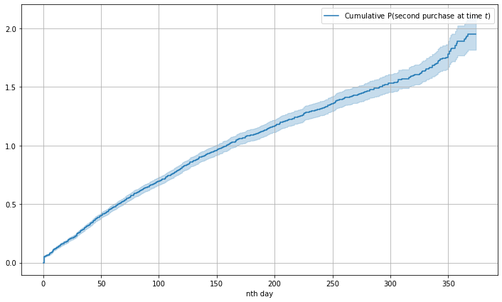
It seems the interpretation would not be too straightforward since now the y-label shows cumulative probabilities of second purchase at \(t\) instead of just probabilities. But at least there are some takeaways. The cumulative hazard increase rate looks quite consistent along the timeline. No interesting sudden rate change at any point \(t\), except in the beginning and the end. Other cumulative hazard functions can have sudden changes in some certain period.
What if we just want to observe the probability? Well, we can now plot the hazard function.
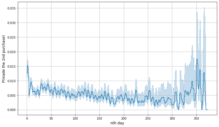
Note that since we’re not deriving the hazard function from our survival function, the hazard function above is estimated from the change rates happened in the cumulative hazard function. Appearantly, the line is more jagged. We see that the probability of second purchase is quite flat along the timeline, but there are notable spikes in the beginning and the end of the timeline, just like we’ve seen on the cumulative hazard plot. While the y-label is more obvious to interpret than the cumulative hazard function, it seems that we won’t need to observe hazard rate at a certain \(t\) that often. Thus, cumulative hazard function is said to be more recommended.
Based on some findings above, looks like we need to give customers more time to deciding on making second purchase. Since our data are based on gift product retail transactions, judging from the product type seems reasonable to expect a customer to not having another purchase at a very short time. Though hopefully we see more interesting survival and hazard function in another problem.
Should you find survival analysis is exciting, have more sneak peek in this course.