There are several purposes of applying dimensionality reduction into a dataset. We often times need to communicate our high-dimensional dataset into a simpler visualization, either in 2D or 3D. Sometimes our model training seems very slow because of the number of features or the size of the data. Sometimes we just need to drop some unnecessary details and noise from our data.

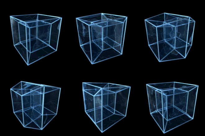
Source: Wiktionary
If you’re someone who have been taking benefits from dimensionality reduction, you might need to revisit the implementations you’ve done for a while. In many cases, this technique can be very advantageous, but in some others, it turns out that there would some pitfalls in applying PCA for certain problems.
Let’s talk about Principal Component Analysis (PCA) as a matter of problem framing. Suppose that you’d like to reduce our dataset dimensionality in order to reduce the training duration of your linear regression model. You’re planning to do so because previously your model got relatively unacceptable training duration. The model seemed also to only work well in the training set.
While implementing PCA, you suddenly recall about how reducing features from \(n\) to \(k\) features could simplify the model and help avoiding overfitting. You also wonder how PCA could help you find the so-called “most important features” to predict your label. You then proceed your PCA implementation and finally obtain the principal components.
With something you reflected about a while ago, you then re-train your model with the PCA-reduced dataset. You get an idea to come up with this comparison (just for an illustration).
| |
Before PCA |
After PCA |
| Training duration |
5.51s |
0.30s |
| R-squared (train) |
0.89 |
0.797 |
| R-squared (val) |
0.395 |
0.77 |
| MSE (train) |
1.084 |
4.817 |
| MSE (val) |
11.61 |
4.806 |
Looks like it actually helps to achieve a faster training. Although there is a performance decrease, the overfitting issue seemed to have been resolved.
Well, what could have gone wrong here?

When we apply PCA to our training set, most likely we do not include our label as a consideration. Simply put, if you’re using PCA class in scikit-learn, you don’t fit() the model into your label together with the features. Well, it is an unsupervised learning technique. Only the features will be mapped from, say, \(X\) features to \(Z\) principal components. The label is ignored by the algorithm.
As the result, our dimensionality reduction algorithm doesn’t know any relationship between our features and our label in the training set. It didn’t find these principal components based on your label. They were based on how the projected axes will maximize the variance retained from our original dataset.
In other words, the principal components (PC) that we got aren’t directly associated with the label you would like to predict. Even if we now have way less PC than our initial features, PCA can’t be considered as a good strategy to avoid overfitting. If we coincidentally got a prediction improvement after training our supervised model with PCA-reduced dataset, it doesn’t mean that our PC are the “most important features” in that particular case.

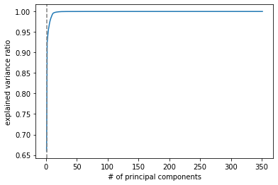
Even if a small numbers of principal components can retain 95% information, there's no guarantee for prediction later.
Also, PCA could throw some meaningful information which can supposedly help making prediction. That’s why in some cases, a model would just perform worse after being trained with PCA-reduced dataset, even with fairly high retained variance.
Having said that, it doesn’t mean that re-training a supervised model with PCA-reduced dataset isn’t allowed at all. However, one should alter his/her thinking process of implementing dimensionality reduction. Instead of to obtain “the most important features” for supervised learning, just intend to reduce the data size in order to shorten the training duration or visualization matters, for instances.
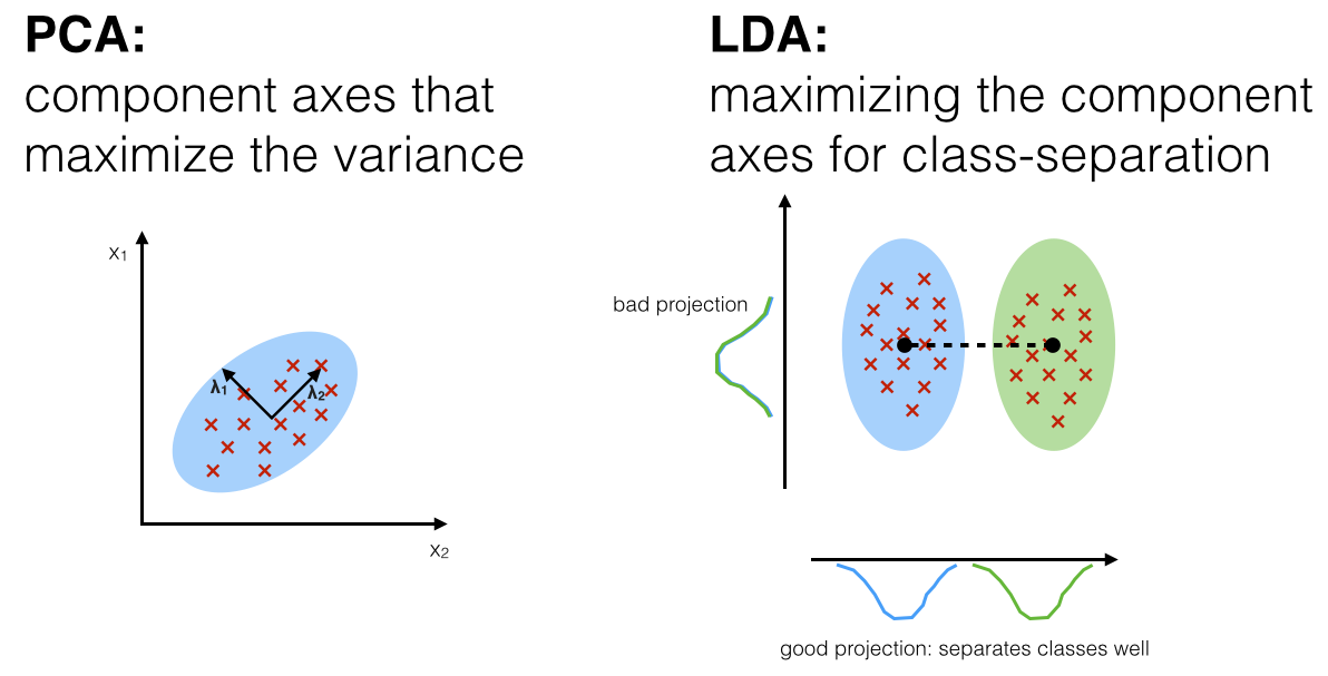
In classification problem, we can consider something like Linear Discriminant Analysis (LDA), which unlike PCA, LDA considers the classes when doing the transformation. It computes the axes that will maximize the class separation, so if you visualize your principal components afterwards, for instance, you would get distinguishable data points between classes.

Source: sebastianraschka.com
If your main concern is still about overfitting, you can use regularization instead.
\[J(\theta) = MSE(\theta) + \alpha\frac{1}{2}\sum_{i=1}^{n}\theta_i^2\]
Ridge regression cost function
As we might know, the regularization term is added to the cost function which is associated with the predicted label.
Oh yes, we only need to apply PCA to our training set, but the same mapping (or parameters) obtained from the training can be re-applied to our validation or test set.
If this short explanation is not digestible enough for you, see how Andrew Ng explains the very same issue in his Machine Learning course in Coursera.
Other reference: